BuildingLoads

Basic

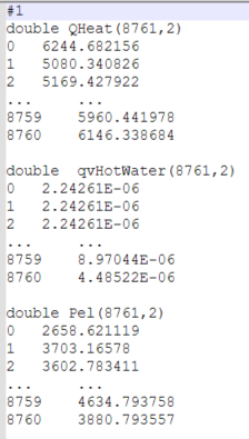
For the load data import the path to the text file must be specified by the parameter File. The table names (names of the values columns within the text file) for the heating, hot water and power loads have to be set by the parameters TableHeat, TablePower and TableDomWater.
An example of an appropriate text file is shown in the screenshot below. The first column is the time in hours and can be as highly resolved as required. The second column contains the values in SI units (power in watts, volume flow in m³/s). In the table header, the table dimensions (number of rows, number of columns) must be indicated in brackets after the table name.

The timebase of the load table can either be supplied in hours of year (useDayTime=false) or in hours of a day (useDayTime=true). Using the latter format, simulations longer than a day will repeat the given load curve accordingly.

The power consumption table values are interpreted as effective power. Positive values are interpreted as power demand and negative values as power supply.

The values of TableHeat represent a heating or cooling load. Based on this the required volume flow (i.e. to cover the demand load) of a heating or cooling medium is calculated using the following equation:

To solve this equation a return temperature is required. Thus a reference temperature is set with parameter TRefReturnHeat as an absolute value. To prevent high volume flows, a minimum temperature difference between flow and return temperature is defined inside the component compound to 1K (it can be changed in parameter dialogue of the component Heating inside the compound with the parameter deltaTMin under the tab hydronic system configuration). The model equation will always use the maximum temperature difference between TFlow and TRefReturn or deltaTMin.

For domestic water consumption the internal water tap works as a heat exchanger heating cold water to the defined tap water temperature (parameter TDomWaterRef) utilizing available heating energy. The default cold water temperature of 10°C can be changed by parameter TColdWater in the parameter dialogue of the component DomesticWater inside the model compound. Heating losses of the hot water distribution and circulation are considered via the parameter eta.

Furthermore, the model can add simple heat pump functionality for both heat and domestic water supply. In case of low temperature district-heating grids, the lower grid heat is elevated to a higher temperature level via a heat pump. Instead of the full heating power required, only the source power is then drawn from the connected heat supply. The required power input is defined via the parameters COPHeating, COPDomWater, cosPhiHeating and cosPhiDomWater, respectively. Both heat pump options can be individually activated via parameters HPHeating and HPDomWater. The required heat pump power demand is automatically added to the existing 3-phase low-voltage grid inside the compound.

The Connector ▶EnvironmentConditions has to be connected to an Environment block to provide the current time of year and time of day for reading the text file. The ▶Flow and ▶Return connectors should be connected to a heat supply system (ideally indirectly via a storage tank). The connected heating supply should define the flow temperature. The volume flow and return temperature are calculated by the DomesticWaterLoad component. If the component has been parameterized for calculation with a heat pump, the electrical connection ▶LVGrid must be connected to an electrical power supply.